Course description

Laws of motion: Newton's first law - It states that every object will remain at rest or in uniform motion in a straight line unless compelled to change its state by the action of an external force. This is normally taken as the definition of inertia. The key point here is that if there is no net force acting on an object (if all the external forces cancel each other out) then the object will maintain a constant velocity. If that velocity is zero, then the object remains at rest. If an external force is applied, the velocity will change because of the force. This means that there is a natural tendency of objects to keep on doing what they are doing. All objects resist changes in their state of motion.

The first law can be stated mathematically when the mass is a non-zero constant, as,

This is known as uniform motion. Moreover, the First Law is just a special case of the Second Law for which the net external force is zero.

Centripetal Force Example: In Fig. 16, the string must provide the necessary centripetal force to move the ball in a circle. If the string breaks, the ball will move off in a straight line. The straight-line motion in the absence of the constraining force is an example of Newton's first law. The example here presumes that no other net forces are acting, such as horizontal motion on a frictionless surface. The vertical circle is more involved.

                                                        Fig. 16                                        

Newton's Second law - Acceleration is produced when a force acts on a mass. The greater the mass (of the object being accelerated) the greater the amount of force needed (to accelerate the object). Therefore, second law explains how the velocity of an object changes when it is subjected to an external force. The law defines a force to be equal to change in momentum (mass times velocity) per change in time. Newton also developed the calculus of mathematics, and the "changes" expressed in the second law are most accurately defined in differential forms. (Calculus can also be used to determine the velocity and location variations experienced by an object subjected to an external force.) For an object with a constant mass m, the second law states that the force F is the product of an object's mass and its acceleration a:

F = ma

For an external applied force, the change in velocity depends on the mass of the object. A force will cause a change in velocity; and likewise, a change in velocity will generate a force. The equation works both ways.

F=dp/dt=(d(mv))/dt=ma

It does not apply directly to situations where the mass is changing, either from loss or gain of material, or because the object is traveling close to the speed of light where relativistic effects must be included. It does not apply directly on the very small scale of the atom where quantum mechanics must be used.

Newton's Second Law Illustration: Newton's 2nd Law enables us to compare the results of the same force exerted on objects of different mass.

                                                 Fig. 17

Newton's Third Law - The third law states that for every action (force) in nature there is an equal and opposite reaction. In other words, if object A exerts a force on object B, then object B also exerts an equal force on object A. Notice that the forces are exerted on different objects. The third law can be used to explain the generation of lift by a wing and the production of thrust by a jet engine.

FA = −FB

                                                  Fig. 18

Problem 6: A mass of 5 kg is suspended by a rope of length 2 m from the ceiling. A force of 45 N in the horizontal direction is applied at the midpoint R of the rope, as shown in Fig. 19. What is the angle the rope makes with the vertical in equilibrium? (Take g = 10 ms-2). Neglect the mass of the rope.

                     Fig. 19

Solution: We begin by drawing the free body diagram of the mass to find T2 (Fig. 20).

As the mass is in equilibrium, the sum of all the external forces on it should be zero.

Therefore, T2 = 50 N. Next, we draw the free body diagram of the point R (Fig. 21).

   Fig. 20                           Fig. 21

Since, point R is also in equilibrium, the sum of all the forces at this point must be zero.

That is, T1 Cosθ = 50 N

and       T1 Sinθ = 45 N   

Therefore, tanθ = (45/50), θ = 420

Frames of Reference:

An arbitrary set of axes with reference to which the position or motion of something is described or physical laws are formulated. However, frame of reference frequently is used to refer to a coordinate system or, even more simply, a set of axes, within which to measure the position, orientation, and other properties of objects. More generally, a frame of reference may include three elements: an observational reference frame, an attached coordinate system, and a measurement apparatus for making observations, as a combined unit.

For example, sometimes the type of coordinate system is attached as a modifier, as in Cartesian frame of reference. Sometimes the state of motion is emphasized, as in rotating frame of reference. Sometimes the way it transforms to frames considered as related is emphasized as in Galilean frame of reference. Sometimes frames are distinguished by the scale of their observations, as in macroscopic and microscopic frames of reference.

Few Common Coordinate Systems:

Number line: The simplest example of a coordinate system is the identification of points on a line with real numbers using the number line. In this system, an arbitrary point O (the origin) is chosen on a given line.

Fig. 22

Cartesian Frame of Reference: A Cartesian coordinate system is a coordinate system that specifies each point uniquely in a plane by a pair of numerical coordinates, which are the signed distances to the point from two fixed perpendicular directed lines, measured in the same unit of length. Each reference line is called a coordinate axis or just axis of the system, and the point where they meet is its origin, usually at ordered pair (0, 0). The coordinates can also be defined as the positions of the perpendicular projections of the point onto the two axis, expressed as signed distances from the origin. In Fig. 23, four points are marked and labeled with their coordinates: (2, 3) in green, (−3, 1) in red, (−1.5, −2.5) in blue, and the origin (0, 0) in purple.

                                  Fig. 23                                                                    Fig. 24

One can use the same principle to specify the position of any point in three-dimensional space by three Cartesian coordinates, its signed distances to three mutually perpendicular planes (or, equivalently, by its perpendicular projection onto three mutually perpendicular lines). Fig. 24 shows a three dimensional Cartesian coordinate system, with origin O and axis lines X, Y and Z, oriented as shown by the arrows. The tick marks on the axes are one length unit apart. The black dot shows the point with coordinates x = 2, y = 3, and z = 4, or (2, 3, 4).

Polar Coordinate System: In mathematics, the polar coordinate system is a two-dimensional coordinate system in which each point on a plane is determined by a distance from a reference point and an angle from a reference direction. The reference point (analogous to the origin of a Cartesian system) is called the pole, and the ray from the pole in the reference direction is the polar axis. The distance from the pole is called the radial coordinate or radius, and the angle is called the angular coordinate, polar angle, or azimuth. Fig. 25 shows the polar coordinate system with pole O and polar axis L. The point with radial coordinate 3 and angular coordinate 60 degrees or (3,60°) and one other point is (4,210°).

                                    Fig. 25

The relationship between polar coordinates r and ϕ and the Cartesian coordinates x and y is:

x=rcosφ

y=rsinφ

Fig. 26 is a diagram illustrating the relationship between polar and Cartesian coordinates. In Fig. 27, (x, y) are the rectangular coordinates and (θ, r) are the polar coordinates.

                                Fig. 26                                                                Fig. 27

Spherical Coordinate Systems: In mathematics, a spherical coordinate system is a coordinate system for three-dimensional space where the position of a point is specified by three numbers: the radial distance of that point from a fixed origin, its polar angle measured from a fixed zenith direction, and the azimuth angle of its orthogonal projection on a reference plane that passes through the origin and is orthogonal to the zenith, measured from a fixed reference direction on that plane. It can be seen as the three-dimensional version of the polar coordinate system. Fig. 28 shows spherical coordinates (r, θ, φ) system: radial distance r, polar angle θ (theta), and azimuthal angle φ (phi). Where the radius or radial distance is the Euclidean distance from the origin O to P. The inclination (or polar angle) is the angle between the zenith direction and the line segment OP. The azimuth (or azimuthal angle) is the signed angle measured from the azimuth reference direction to the orthogonal projection of the line segment OP on the reference plane.

                                                Fig. 28

Cylindrical Coordinate System: A cylindrical coordinate system is a three-dimensional coordinate system that specifies point positions by the distance from a chosen reference axis, the direction from the axis relative to a chosen reference direction, and the distance from a chosen reference plane perpendicular to the axis. The latter distance is given as a positive or negative number depending on which side of the reference plane faces the point. The origin of the system is the point where all three coordinates can be given as zero. This is the intersection between the reference plane and the axis. Fig. 29 shows a cylindrical coordinate system with origin O, polar axis A, and longitudinal axis L. For example, the dot p is the point with radial distance ρ = 4, angular coordinate φ = 130°, and height z = 4.

                            Fig. 29

Relationship between the spherical coordinates (r, θ, φ) and cylindrical coordinates (ρ, φ, z) are:

ρ=rcosθ

z=rsinθ

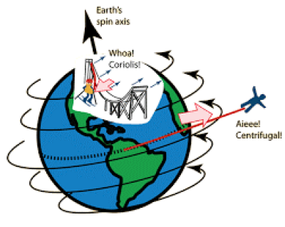
Rotating Frame of Reference:

A rotating frame of reference is a special case of a non-inertial reference frame that is rotating relative to an inertial reference frame. An everyday example of a rotating reference frame is the surface of the Earth. A non-inertial reference frame is a frame of reference that is undergoing acceleration with respect to an inertial frame

                                            Fig 30

Galilean frame of reference: An inertial frame of reference (Galilean reference frame), in classical physics, is a frame of reference in which bodies, whose net force acting upon them is zero, are not accelerated, that is they are at rest or they move at a constant velocity in a straight line. In analytical terms, it is a frame of reference that describes time and space homogeneously, isotropically, and in a time-independent manner. All inertial frames are in a state of constant, rectilinear motion with respect to one another; an accelerometer moving with any of them would detect zero acceleration. Measurements in one inertial frame can be converted to measurements in another by a simple transformation (the Galilean transformation in Newtonian physics and the Lorentz transformation in special relativity). Fig. 31 shows Galilean reference frame and Fig. 32 shows the inertial and rotating of references.

Fig. 31

Fig. 32

What will i learn?